Activity 6: Properties of the 2D Fourier Transform

We seek to understand the properties of the 2D Fourier Transform by applying it to several test cases. Below are the results I've gathered:

ORIGINAL / FFT







square / square annulus / donut / slits / dots









several cases of the sin function:
3 vertical sin waves of decreasing frequencies / biased / rotated / sum of sines in x and y / previous case + rotated sines

Both the FT's of the square and the square annulus look like stars/crosses. They only differ in that the latter looks striped such that it jumps over some values. The symmetry of the FTs reflect the symmetry of the squares. The FT of a donut has a strong peak at the center and is surrounded by a symmetric pattern covering some circular area around it. This reflects the circular symmetry of the object. The FT of the slits looks like a vertical interference pattern at the center. It is as if we have recorded the interference pattern after ltting light pass through the slits. This is expected as the diffraction pattern we get from an aperature is the same its FT.

The FT of the two dots look like the superposistion of two airy disks symmetrically off center. We already found in the previous experiment that the FT of a circle is an airy disk. It is expected then that the FT of two circles is simply a superposition of two airy disks.

As the frequency of the sine wave decreases, the point corresponding to the frequency of the sine wave come closer to the center. As expected, the FT is symmetric along the X axis. Adding a bias simply adds a point at the center of the FT. Rotating the sine wave rotates the FT by the same angle. The last FT turned out as expected since it is simply a superposition of the previous FT's. It outlines a circle since we sum up rotations of the same frequencies. In addition, we still retain the four points from the previous FT.

I give myself a grade of 9/10 because I was able to execute the procedure but I feel I could do better in interpreting the results.

Activity 5: Fourier Transform and Correlation

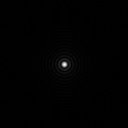
In this activity, we explored the uses of FFT and correlation in image processing. We started by taking the FFT of a circle and a character just to see how the 2D FFT function works in Scilab. I got the following results:

Original/FFT/double FFT
Top: Circle, Bottom: A

These results agree with the analytical expectation: we get an Airy disk for the circle and we inverse the image when the FFT is performed twice.

We then used FFT to convolve an image of an aperature and an image to simulate the effect of an imaging device with limited aperature. I got the following result:

Original image/ Convolution of "VIP" and circular aperature of r=40/30/20/10/5

We get an image of the original object but it is now inverted and less resolved. Decreasing the aperature size causes the image to blur and gain artifacts which somehow resemble the shape of the aperature.

Our next task was to use correlation to find a certain pattern in an image. In this case, we had an image of the line "THE RAIN IN SPAIN STAYS MAINLY IN THE PLAIN" and we had to look for the A's via correlation. Correlating the image and an image of the letter "A", I came up with the following result:

Original image/Correlation of the image and pattern

We find that the peaks of the resulting image correspond to the posistions of the A's in the image thus verifying that the method was correct.

Finally, we attempted to do edge detection by correlating small matrices of either a vertical line, a horizontal line, or a point with a given image. I came up with the following results:

Vertical/horizonal/point edge detection

We can see that the method worked as it highlighted only the parts which correspond to the types of edges being detected.

For this activity I give myself a 10/10 because I was able to complete the tasks completely and efficiently.

Activity 4

In this activity we were tasked to change the improve the contrast of a grayscale image by tweaking it such that its CDF is converted to some desired curve. To do this we took the CDF of the original image then matched the pixel values with the same value on the original CDF and desired. We then edited the image such that every pixel with a given pixel value on the original image is replaced with its matched pixel value from the desired CDF. Here are my results:

BEFORE:

original image 250x250 grayscale

original PDF

original CDF

AFTER:

resulting image 250x250 grayscale

resulting PDF

resulting CDF

The resulting image had much better contrast. The details of the petals and the background are now much more easily distinguishable. The resulting CDF is quite close to the desired (linear). The few kinks on th curve are probably a result of the limitations of histograms. Since histogram values are discrete it is possible that some values on the original CDF dont have corresponding values on a desired CDF. I give myself a 9/10 for this activity because I was able to execute the procedure properly yet I believe that there is room for improvement in the method such that the resulting CDF may be exact.

Activity 2: Area estimation for images with defined edges

In this activity we set out to determine the area of an ROI in a binary image by first tracing its contour then using Green's theorem to calculate the area enclosed. To prepare the image for processing, I first had to convert the image to a binary matrix using the im2bw function. I then used the follow function to trace the ROI's contour. I then implemented the discrete form of green's theorem to finally come up with the area.

After preliminary results Ifound that the area we would calculate was always lacking by half of the contours length. I speculated that the follow function traced the inner contour of the ROI, thus decreasing the area enclosed by some value. M. Sison proposed that to correct the calculated area, we simply add half the length of the contour. After testing the method over various shapes, both regular and irregular, we found the the proposed correction was indeed valid.

Sample Results

Shape 1: 200 x 200 Square

Analytical: 40000 pixels
Pixel count: 40000 pixels
Program: Analytical: 40000 pixels

Shape 2: Robot

Analytical: 32071 pixels
Pixel count: 32701 pixels
Program: 32071 pixels

Shape 3: Irregular

Analytical: N/A
Pixel count: 26526 pixels
Program: 26526 pixels

For this experiment, I give myself a score of 10/10 because I was able to implement the method properly and the results attest to the accuracy of the program.